
Analyzing Crime Data of the City of Los Angeles
Auther: Linchuan Yang(linchuan@ucsb.edu)
Abstract
Crime is happening all over the world all the time, and the City of Los Angeles as a metropolis is even more so. This report will analyze Los Angeles criminal records from 2010 to 2021 to provide readers with a better understanding of crime in the City of Los Angeles. At the same time, the report will also use analytical techniques at the end to show the possible impact of the epidemic on crime victims.
Introduction
Background:
Our project is about analysing and exploring the crime reports of the City of Los Angeles from 2010 to 2021. This project topic is closely related with area of Criminology and Sociology. The data were gathered from the offical data base of the City of Los Angeles which contains every crime reported to the law enforcement with the LA. In the raw dataset, exact time, exact location, area and district where crime performed, crime code and description, and victim information were included.
The motivation for this project is simple, Los Angeles is close to Santa Barbara, only a two-hour drive, which is familiar to us. Also, the observations of Los Angeles are huge which is good for data exploring. Moreover, we choose dataset from 2010 to 2021 because we were interested seeking and informing readers how COVID-19 started in 2020 may affect on crime reported in LA city and get some sense how crime in LA city would be in the future.

Data Sources:
Crime Data from 2010 to 2019: https://data.lacity.org/Public-Safety/Crime-Data-from-2010-to-2019/63jg-8b9z
Crime Data from 2020 to Present: https://data.lacity.org/Public-Safety/Crime-Data-from-2020-to-Present/2nrs-mtv8
Approach:
To analyze the data, we will focus on time, area, crime information, and victim information to answer several specific self-interested questions listed below. Each group member will answer their own questions.
In this project, several data analysis technics are used to answer the questions, including:
Achieving Data, Data Tidying, Visualizing, Plot Analyzing, PCA Analysis, Loess Plot Analysis
Questions:
Visualizing and Plot Analyzing:
- What month throughout the years has the most concentration of crimes happening?
- What age/sex seems to be the least victimized from 2010 to 2021?
- Which area in LA city were considered dangerous?
PCA Analysis:
- List the crime by bigger major categories and apply to the data. Is there any area that different from others?
Loess Plot Analysis:
- How was the trend that a specific descent group were victimlized?
Raw Data
# import packages
import pandas as pd
import numpy as np
The table below shows the raw data. The raw data include all the crime records reported within the City of Los Angeles from 2010 to 2022. The datasets are achieved from the database of City of Los Angeles, the datasets are recorded by Summary Reporting System (SRS) of Division Uniform Crime Reporting (UCR) of Program Criminal Justice Information Services (CJIS) under U.S. Department of Justice. Also, the data are collected from local law enforcement jurisdictions.
# show first five rows
pd.read_csv('data/raw/Crime_Data_from_2010_to_2019.csv').head()
| DR_NO | Date Rptd | DATE OCC | TIME OCC | AREA | AREA NAME | Rpt Dist No | Part 1-2 | Crm Cd | Crm Cd Desc | … | Status | Status Desc | Crm Cd 1 | Crm Cd 2 | Crm Cd 3 | Crm Cd 4 | LOCATION | Cross Street | LAT | LON | |
|---|---|---|---|---|---|---|---|---|---|---|---|---|---|---|---|---|---|---|---|---|---|
| 0 | 1307355 | 02/20/2010 12:00:00 AM | 02/20/2010 12:00:00 AM | 1350 | 13 | Newton | 1385 | 2 | 900 | VIOLATION OF COURT ORDER | … | AA | Adult Arrest | 900.0 | NaN | NaN | NaN | 300 E GAGE AV | NaN | 33.9825 | -118.2695 |
| 1 | 11401303 | 09/13/2010 12:00:00 AM | 09/12/2010 12:00:00 AM | 45 | 14 | Pacific | 1485 | 2 | 740 | VANDALISM – FELONY ($400 & OVER, ALL CHURCH VA… | … | IC | Invest Cont | 740.0 | NaN | NaN | NaN | SEPULVEDA BL | MANCHESTER AV | 33.9599 | -118.3962 |
| 2 | 70309629 | 08/09/2010 12:00:00 AM | 08/09/2010 12:00:00 AM | 1515 | 13 | Newton | 1324 | 2 | 946 | OTHER MISCELLANEOUS CRIME | … | IC | Invest Cont | 946.0 | NaN | NaN | NaN | 1300 E 21ST ST | NaN | 34.0224 | -118.2524 |
| 3 | 90631215 | 01/05/2010 12:00:00 AM | 01/05/2010 12:00:00 AM | 150 | 6 | Hollywood | 646 | 2 | 900 | VIOLATION OF COURT ORDER | … | IC | Invest Cont | 900.0 | 998.0 | NaN | NaN | CAHUENGA BL | HOLLYWOOD BL | 34.1016 | -118.3295 |
| 4 | 100100501 | 01/03/2010 12:00:00 AM | 01/02/2010 12:00:00 AM | 2100 | 1 | Central | 176 | 1 | 122 | RAPE, ATTEMPTED | … | IC | Invest Cont | 122.0 | NaN | NaN | NaN | 8TH ST | SAN PEDRO ST | 34.0387 | -118.2488 |
5 rows × 28 columns
Data Tidying
The table below shows the tidied data. The tidied data only include need variables for the analysis like Year, Month, Crime description, and Victim information.
# show first five rows
pd.read_csv('data/Crime_Data_from_2010_to_Present_Clean.csv').head()
| Month | Year | Area | Crime | Victim Age | Victim Sex | Victim Descent | |
|---|---|---|---|---|---|---|---|
| 0 | 2 | 2010 | Newton | VIOLATION OF COURT ORDER | 48 | Male | Hispanic |
| 1 | 9 | 2010 | Pacific | VANDALISM – FELONY ($400 & OVER, ALL CHURCH VA… | Unknown | Male | White |
| 2 | 8 | 2010 | Newton | OTHER MISCELLANEOUS CRIME | Unknown | Male | Hispanic |
| 3 | 1 | 2010 | Hollywood | VIOLATION OF COURT ORDER | 47 | Female | White |
| 4 | 1 | 2010 | Central | RAPE, ATTEMPTED | 47 | Female | Hispanic |
The table below shows the variable descrition of tidied data.
| Name | Variable description | Type | Units of measurement |
|---|---|---|---|
| Month | ith month | Numeric | Calendar month |
| Year | year of crime record | Numeric | Calendar year |
| Area | specific area where crime occurred | Text | — |
| Crime | crime describtion | Text | — |
| Victim Age | the age of victim | Numeric | years old |
| Victim Sex | the sex of victim | Text | — |
| Victim Descent | the descent of victim | Text | — |
Data Visualization
Initial Visualization
This section will show basic informative plot of the cirme data of the City of Los Angeles.
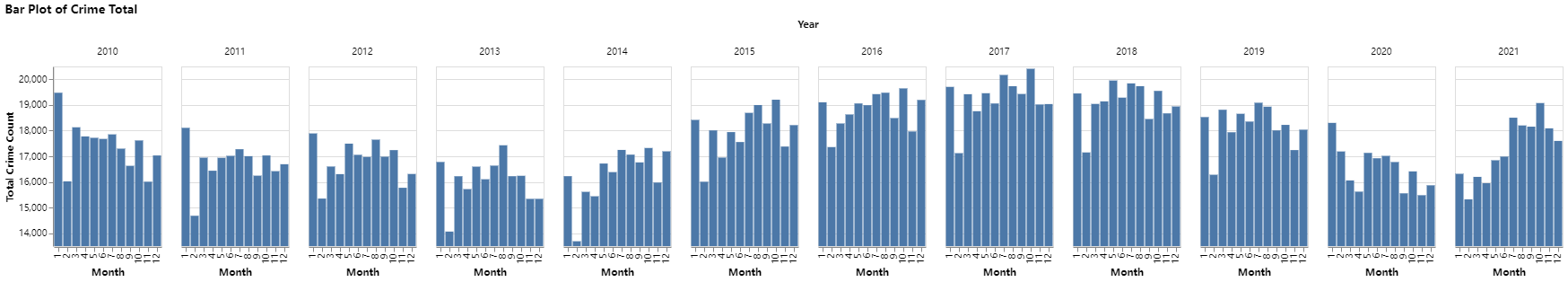
Bar Plot of Crime Total
The bar plot below shows the crime numbers on each month in each year and how they were distributed, minor seasonal trend were observed.
Pie Chart of Victim Descent by Year
The pie chart below shows the victim numbers of each year by descent, increasing trend on Asian Victim proportion were observed.

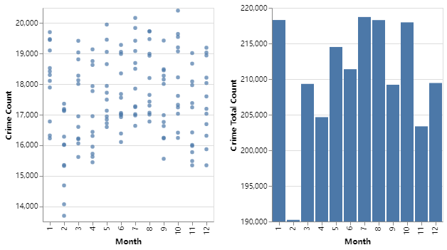
(Question 1) What month throughout the years has the most concentration of crimes happening?
The plot below suggests that Janurary, July, Auguest, and October have the most concentration of crimes happening.
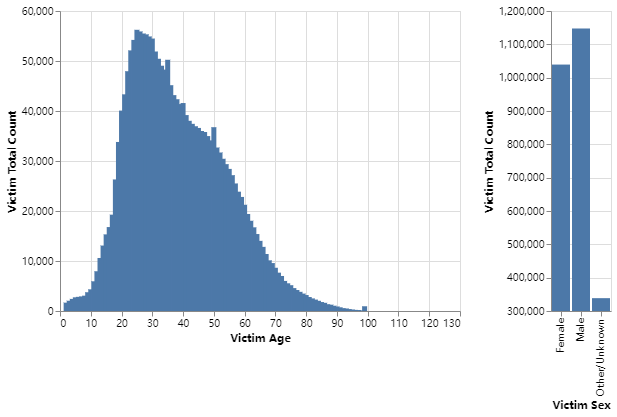
(Question 2) What age/sex seems to be the least victimized from 2010 to 2021?
The plot below suggests that before adult and elder people were least victimized from 2010 to 2021.
Also, other genders and female are less vicimized from 2010 to 2021.
Notice, this does not means that these groups are overally less victiimized because the populations are different. Proper weight need to be added in order to reflect reality.
(Question 3) Which area in LA city were considered dangerous?
Description:
The acreage data are collected by going through each ditrict information from offical LAPD website. Then a data frame with area and acreage are created and merge with crime data grouped by Year and Area. After that, the index is calculated by Crime divide by Acreage then store to the merged data frame with variable name Dangerous Index. Finally, plot the bar plot of Dangerous Index with Area.
Create Plot Dataframe:
# display first five rows
pd.read_csv('data/table/area_acreage_crime_data.csv').head()
| Year | Area | Crime | Acreage | Dangerous Index | |
|---|---|---|---|---|---|
| 0 | 2010 | 77th Street | 14441 | 11.9 | 1213.529412 |
| 1 | 2011 | 77th Street | 14257 | 11.9 | 1198.067227 |
| 2 | 2012 | 77th Street | 14300 | 11.9 | 1201.680672 |
| 3 | 2013 | 77th Street | 13746 | 11.9 | 1155.126050 |
| 4 | 2014 | 77th Street | 14065 | 11.9 | 1181.932773 |
Result:

From the plot above, we observed that 77th Street area has the highest dangerous index which means 77th Street tend to be the most ‘dangerous’ area of the City of Los Angeles.

Also, Hollenbeck and Foothill area has the lowest dangerous index which means Hollenbeck and Foothill tend to be the ‘safest’ area of the City of Los Angeles.


It is also interesting that from the map, 77th Street is at urban area while Hollenbeck and Foothill are at rural area. It make some sense that urban area tend to have higher crime rate and vice versa.
Moreover, the plot also explains the difference of dangerous index is not significance through Year of each area to avoid paradox.
Noice the dangerous index is only based on acreage and crime count of the each area which means it might not be fully correctly refelct the reality.
Data Source: https://www.lapdonline.org/lapd-organization-chart/
PCA Analysis
(Question 4) List the crime by bigger major categories and apply to the data. Is there any area that different from others?
Description:
In order to find the bigger category of the crimes, PCA analysis is required. But first, we will have to transform the data with each crime as a column and value as the count of the crimes. After that, draw a heat map and see weather there are strong corrlations among each crime variables. Then, normalize the matrix data and compute PCs. And then, plot the variance explained graph and decide the number of PCs. After that, analyse the PCs with a loading plot and try to make sense on these PCs. Finally, apply PCs back to the original data and examine the questions.
Data Transform:
# display first five rows
pd.read_csv('data/table/pca_data.csv').head()
| Month | Year | Area | Crime_ABORTION/ILLEGAL | Crime_ARSON | Crime_ASSAULT WITH DEADLY WEAPON ON POLICE OFFICER | Crime_ASSAULT WITH DEADLY WEAPON, AGGRAVATED ASSAULT | Crime_ATTEMPTED ROBBERY | Crime_BATTERY – SIMPLE ASSAULT | Crime_BATTERY ON A FIREFIGHTER | … | Crime_UNAUTHORIZED COMPUTER ACCESS | Crime_VANDALISM – FELONY ($400 & OVER, ALL CHURCH VANDALISMS) | Crime_VANDALISM – MISDEAMEANOR ($399 OR UNDER) | Crime_VEHICLE – ATTEMPT STOLEN | Crime_VEHICLE – MOTORIZED SCOOTERS, BICYCLES, AND WHEELCHAIRS | Crime_VEHICLE – STOLEN | Crime_VIOLATION OF COURT ORDER | Crime_VIOLATION OF RESTRAINING ORDER | Crime_VIOLATION OF TEMPORARY RESTRAINING ORDER | Crime_WEAPONS POSSESSION/BOMBING | |
|---|---|---|---|---|---|---|---|---|---|---|---|---|---|---|---|---|---|---|---|---|---|
| 0 | 1 | 2010 | 77th Street | 0 | 4 | 0 | 88 | 16 | 160 | 0 | … | 0 | 46 | 58 | 4 | 0 | 92 | 15 | 10 | 0 | 0 |
| 1 | 1 | 2010 | Central | 0 | 1 | 0 | 29 | 5 | 109 | 0 | … | 0 | 14 | 15 | 0 | 0 | 17 | 3 | 4 | 0 | 0 |
| 2 | 1 | 2010 | Devonshire | 0 | 1 | 0 | 15 | 2 | 65 | 0 | … | 0 | 42 | 54 | 2 | 0 | 71 | 12 | 5 | 0 | 0 |
| 3 | 1 | 2010 | Foothill | 0 | 1 | 0 | 32 | 1 | 56 | 0 | … | 0 | 43 | 41 | 1 | 0 | 75 | 1 | 20 | 0 | 0 |
| 4 | 1 | 2010 | Harbor | 0 | 3 | 0 | 14 | 8 | 48 | 0 | … | 0 | 40 | 42 | 1 | 0 | 84 | 31 | 2 | 0 | 0 |
5 rows × 146 columns
Correlation Heat Map:

From the heat map above, some strong correlations between crimes are observed.
Select PCs:
The table and the plot below show the proportion and cumulative variance explained by PC components.
# read table
pd.read_csv('data/table/pca_var_explained.csv').head(6)
| Proportion of variance explained | Component | Cumulative variance explained | |
|---|---|---|---|
| 0 | 0.071215 | 1 | 0.071215 |
| 1 | 0.046773 | 2 | 0.117988 |
| 2 | 0.037056 | 3 | 0.155044 |
| 3 | 0.027385 | 4 | 0.182429 |
| 4 | 0.018890 | 5 | 0.201319 |
| 5 | 0.013008 | 6 | 0.214327 |

From the plot, we can see that first 6 PCs are good for analyzing with cumulative 0.214327 of total variance explained.
However, 6 PCs are too complicated to analyse, we will use first 4 PCs for analyzing with cumulative 0.182429 of total variance explained.

From the loading plot, we can see PC1 is more likey to be firearm related crime. PC2 is more likey thefting and transpassing. PC3 is more likey assulting and GTA. PC4 is more likey other than theft and burglary.
PCA Transform:
The table below shows the project data after PCA transform.
# read table
pd.read_csv('data/table/pca_projected_data.csv').head()
| PC1 | PC2 | PC3 | PC4 | Month | Year | Area | |
|---|---|---|---|---|---|---|---|
| 0 | 8.637380 | -6.726617 | 6.533671 | -3.985459 | 1 | 2010 | 77th Street |
| 1 | -1.842980 | -1.912674 | 1.033121 | 5.089348 | 1 | 2010 | Central |
| 2 | -2.953900 | -2.030991 | 2.143411 | -4.391370 | 1 | 2010 | Devonshire |
| 3 | 0.324112 | -4.114268 | 1.741791 | -3.037902 | 1 | 2010 | Foothill |
| 4 | 0.851694 | -5.157373 | 1.653398 | -1.814922 | 1 | 2010 | Harbor |
Outliers:
The plot and table below show the outliers of PC2(Thefting and Transpassing) and PC3(Assulting and GTA).

pd.read_csv('data/table/pc2_pc3_outliers.csv')
| PC1 | PC2 | PC3 | PC4 | Month | Year | Area | |
|---|---|---|---|---|---|---|---|
| 0 | 1.769598 | 7.507764 | 7.523993 | 5.449909 | 1 | 2019 | Central |
| 1 | 0.617683 | 7.582819 | 6.898608 | 6.013018 | 4 | 2018 | Central |
| 2 | 2.322512 | 6.917347 | 7.569194 | 5.929423 | 5 | 2019 | Central |
| 3 | 2.629848 | 7.763640 | 7.114979 | 4.595560 | 6 | 2019 | Central |
| 4 | 2.997893 | 7.276762 | 7.067218 | 4.470929 | 7 | 2019 | Central |
| 5 | 3.572977 | 8.699017 | 6.278390 | 4.077510 | 8 | 2019 | Central |
| 6 | 4.568350 | 9.548046 | 6.421643 | 5.387357 | 9 | 2019 | Central |
| 7 | 2.886755 | 10.791482 | 4.462664 | 4.401455 | 11 | 2021 | Central |
Result:
From the PCA Analysis, the bigger major categories of crimes are firearm related category, thefting and transpassing category, assulting and GTA category, and other than theft and burglary category.
Since there are no obvious outliers formed with each two PCs, we will take look into place and time with high Assulting, GTA, Thefting and Transpassing crime catagories, and assume them as outliers. From the outliers listed above, we can see Central area in 2019 different from the other area tend to have more Assulting, GTA, Thefting and Transpassing than the other time in other area.
Loess Plot Analysis
How was the trend that a specific descent group were victimlized?
Description:
From Pie Chart of Victim Descent by Year in Initial Visualization, we can see that there are trend that some specific descent group were becoming more or less victimlized. To analyse the trend, we will go deeply by month and do a Loess Plot Analysis.
Table of Victim Descent by Month:
# read table
pd.read_csv('data/table/victim_descent_data.csv').head()
| Year | Month | Victim Descent | Proportion | |
|---|---|---|---|---|
| 0 | 2010 | 1 | American Indian | 0.0006 |
| 1 | 2010 | 1 | Asian | 0.0339 |
| 2 | 2010 | 1 | Black | 0.1951 |
| 3 | 2010 | 1 | Hispanic | 0.4569 |
| 4 | 2010 | 1 | Pacific Islander | 0.0004 |
Scatter Plot:

From the plot above, we observed the proportion of Asian are incresingly to be victimlized while the other descents were dropping at 2020 to 2021. So lets take a look from 2018 to 2021.

From the plot above, we observed that the proportion of Victim descents after 2019 are more vibrating than before. To get better understanding on trend, loess plot or multi-linear gression is required. However, since the pattern is seasonal instead of linear, we cannot use multi-linear gression. Therefore, loess plot will be apply for this question.

From the loess plot above, we observed that the proportion of Asian being victimlized are countinuous increasing from June 2020 while the proportion of other desent are bouncing seasonally.
One potential reason explains why Asian descent are tend to more likely being victimlized is “Asian Hate” leaded by “COVID-19”.
As “Covid ‘hate crimes’ against Asian Americans on rise” from BBC News stated, from March to May 2020 alone, over 800 Covid-related hate incidents were reported from 34 counties in the state, according to a report released by the Asian Pacific Policy Planning Council.

Source: https://www.bbc.com/news/world-us-canada-56218684
Also, Notice that since the analysis is based on the proportion of descent being victimlized. Correlation may interact with each other, which mean, the incerase of proportion may not because of actual increase, may also because the decrease of other proportion and vice versa. So that the result may not fully reflect reality.
Discussion
From the all the analysis above, we can draw conclusions on each part.
From visualization part, we can observed that Janurary, July, Augest and October are the most concentrated Months with crimes happening. Also, age 20 to 30 are the most population being victimlized. Moreover, male victims are more than female victims. At last, with visual analysis on dangerous index, we derived that 77th Street Area is considered most dangerous area, on the other hand, Hollenbeck and Foothill area are considered safest area in the City of Los Angeles.
From PCA analysis part, by using PCA from sklearn package, four major bigger categories of crimes are discovered. The four major bigger categories are firearm related category, thefting and transpassing category, assulting and GTA category, and other than theft and burglary category. Also, analysis has pointed out that Central area in 2019 different from the other area tend to have more Assulting, GTA, Thefting and Transpassing than the other time in other area of the City of Los Angeles.
From Loess polt analysis part, by plotting the loess plot of victim count by descent, we found a potential increase on proportion of Asian descent. Connect to the new about COVID-19 related Asian Hate, the findings also make sense to the reality.
For future, since significant bouncing pattern on victim descent scatter plot observed after COVID-19 transmitted to the City of Los Angeles. Will the scatters still keep this pattern for post-COVID time, or will the pattern get back to normal? This question will be very thought-provoking for future analysis on crime data.